Every capital number comes out of a model. Not out of the book of business — out of a model of the book. Everyone in the room knows the model is wrong; the argument is only ever about how wrong, and whether it matters. Usually that argument ends with a margin: some percentage, set years ago, defended in a memo nobody can find.
This post runs the argument with arithmetic instead. The plan has three steps. First, say in dollars how far from the truth our loss model could plausibly be. Second, consider every distribution that close to our model — not a handful of hand-built stress scenarios, all of them. Third, report the worst capital requirement any of them produces. Step two sounds impossible. It turns out to be a one-line formula.
The tool is robustvalue, from the optimal-transport toolkit in ActuaryUtilities.jl. The previous post, How Far Did the Book Move?, used the toolkit’s other three functions to measure a stop-loss book’s severity drift. You do not need to have read it — everything here is explained from scratch — but the book is the same one, and the numbers carry over.
The book, briefly
Two simulated policy years of a stop-loss claimant file. Each row is one claimant’s ground-up claims for the year, and the carrier reimburses whatever part of each total exceeds a $250,000 deductible. Because the data are simulated, we know the truth exactly: claims come from the mixture laws written out in the code below, and the current year really is worse than the prior one — more cost, thicker tail. To each year we fit the model a busy pricing actuary might actually use, a single lognormal. The fit is deliberately imperfect. That is the point. We are about to charge for the imperfection.
setup and the book from part one (same code, same seeds)
using ActuaryUtilities, Distributions, DataFrames, Statistics, Random, Printf
using CairoMakie

# site plot theme (cassette futurism)
include(joinpath(@__DIR__, "..", "..", "assets", "themes", "cassette_futurism.jl"))
set_theme!(cassette_futurism_theme())

# formatting helpers for prose and tables
comma(x) = replace(@sprintf("%.0f", x), r"(?<=[0-9])(?=(?:[0-9]{3})+$)" => ",")
usd(x) = "\$" * comma(x)
musd(x) = @sprintf("\$%.1fM", x / 1e6)
pct1(x) = @sprintf("%+.1f%%", 100x)

prior_law = MixtureModel(
    [LogNormal(log(62_000), 0.95), LogNormal(log(650_000), 0.55)],
    [0.960, 0.040])
current_law = MixtureModel(
    [LogNormal(log(62_000) + log(1.085), 0.97), LogNormal(log(650_000) + log(1.085), 0.55)],
    [0.945, 0.055])
claims_prior = rand(Xoshiro(1001), prior_law, 1620)     # prior policy year
claims_current = rand(Xoshiro(2001), current_law, 1775) # current policy year
ded = 250_000

fit_prior = fit_mle(LogNormal, claims_prior)
fit_current = fit_mle(LogNormal, claims_current)

w1 = wasserstein(claims_prior, claims_current)          # a year of drift, per claimant
misfit = wasserstein(fit_current, claims_current)       # model error, per claimant
basis_move = wasserstein(fit_prior, fit_current)        # a year of drift, basis to basis

DataFrame([
    (year = "prior", n = length(claims_prior), mean = usd(mean(claims_prior)),
        fitted_basis = @sprintf("LogNormal(%.3f, %.3f)", fit_prior.μ, fit_prior.σ)),
    (year = "current", n = length(claims_current), mean = usd(mean(claims_current)),
        fitted_basis = @sprintf("LogNormal(%.3f, %.3f)", fit_current.μ, fit_current.σ)),
])
| Row |
year |
n |
mean |
fitted_basis |
|
String |
Int64 |
String |
String |
| 1 |
prior |
1620 |
$125,986 |
LogNormal(11.155, 1.036) |
| 2 |
current |
1775 |
$151,514 |
LogNormal(11.262, 1.094) |
Two measurements from part one set the scale of the problem, and both come from the same simple idea, so here it is in one breath. To measure how far apart two loss distributions are: line both up smallest to largest, match them rank for rank — smallest with smallest, median with median, worst with worst — and average the dollar gaps between partners. That average is the Wasserstein distance. It is the cost, in dollars per claimant, of rearranging one distribution into the other. Not a test statistic, not a p-value. A moving bill.
By that ruler, the fitted lognormal misses the very claims it was fitted to by $20,039 per claimant. And the fitted model moved $21,776 per claimant between last year’s fit and this year’s. Read those together: on this dollar ruler, model misfit is about as large as one year of basis movement. Whether the two matter equally is a separate question — a distance says how much probability moved, not where, and tails and layers care where — but the order of magnitude is the point. The error we ignore by trusting the model is the size of an error nobody would knowingly ignore: pricing on a year-old book. This post is about pricing it instead.
Capital lives in the aggregate
Part one worked claimant by claimant. Capital does not. A capital requirement attaches to the whole year at once: how many claimants show up, times what each one costs, keeping only the part above the deductible. So we need an annual aggregate loss model, and ours is the ordinary textbook one. Claim counts are Poisson, centered on the current year’s volume. Each claim is a draw from the fitted lognormal. The carrier pays each claimant’s excess over $250,000, and the year’s total ceded loss is the number we track.
Count the assumptions in that paragraph: Poisson counts, independent claims, frequency frozen at this year’s level, and severities from a lognormal we just measured missing by $20,039 a head. None of this is embarrassing — it is how capital models are actually built. But every item is a choice, and for the last one we hold the error in dollars. Keep that number in view. The rest of the post is about what it costs.
One definitional note before any formulas. The standard we will price is \(\text{CTE}_\alpha\) of the annual ceded loss — the average of the worst \(1-\alpha\) share of years. Strictly, that is a required-asset level: a provision against the year’s loss. It is not quite economic capital, which in most frameworks is this provision minus whatever expected loss, premium, or reserve is already funded against it. We stay with the provision throughout, because it is the quantity the robust theorem prices exactly. Netting a funded amount off afterward is simple subtraction — but the worst case of a difference over a ball of models is a different optimization, and this post does not solve that one.
function aggregate_ceded(rng, sev_law, λ, d, nsims)
    map(1:nsims) do _
        sum(max(rand(rng, sev_law) - d, 0.0) for _ in 1:rand(rng, Poisson(λ)); init = 0.0)
    end
end

λ = length(claims_current)   # claimants per policy year, held fixed across bases
agg_prior_basis = aggregate_ceded(Xoshiro(11), fit_prior, λ, ded, 40_000)
agg_current_basis = aggregate_ceded(Xoshiro(12), fit_current, λ, ded, 40_000)

println("aggregate ceded mean: prior basis ", musd(mean(agg_prior_basis)),
    " → current basis ", musd(mean(agg_current_basis)))
aggregate ceded mean: prior basis $41.4M → current basis $64.7M
How wrong could we be? Let last year answer
To charge for model error we need one number first: a dollar budget for how far from the truth the model might sit. The code calls this number the radius — the picture behind the name arrives in the next section — and nothing in mathematics will choose it for us. Once it is chosen, the worst-case arithmetic downstream is exact, conditional on the distribution we apply it to. So we want an anchor everyone can see, and history offers one.
Here is the logic behind that anchor, spelled out, because it is easy to miss. A capital model is never estimated on the year it is used for: you fit on data through the last cycle and apply the result to the next one. And part one established that this book genuinely moves between cycles. Put those two facts together. At the moment the model is used, it is already wrong by at least however far the book has moved since the data it was fitted on — even if the fitting were flawless. Staleness is not an exotic failure mode; it is the default one. So “how wrong could our model be?” contains a measurable special case: “how wrong does one cycle of staleness make it?” That one, our own filing cabinet can answer.
We hold two fitted models: last year’s and this year’s. Run the identical aggregate machine under each — same counts, same deductible, only the severity model swapped — and we get two versions of the annual loss distribution: what the model said a year looked like then, and what it says now. Then measure the distance between those two annual distributions, with the same sorting idea as before and one small change: square the gaps before averaging, then un-square at the end. Squaring makes the distance pay extra attention to large rearrangements. That version is called \(W_2\); the plain average is \(W_1\). The formula coming in the next section is built for \(W_2\), so that is what we compute:
radius = wasserstein(agg_prior_basis, agg_current_basis; p = 2)
println("W₂ between the two aggregate laws (one repricing cycle of drift): ", musd(radius))
W₂ between the two aggregate laws (one repricing cycle of drift): $23.4M
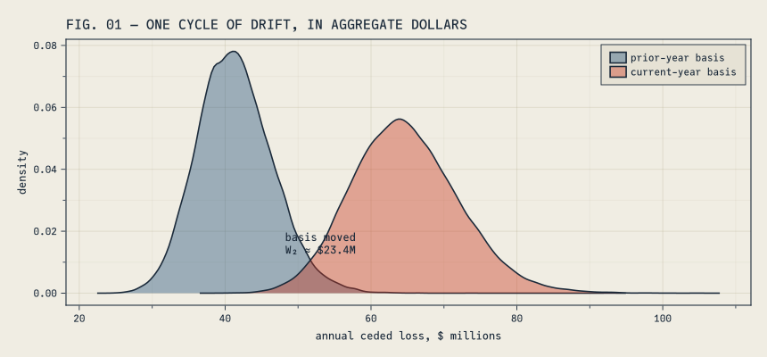
(For these two distributions the squaring hardly matters — \(W_2\) comes to $23.4M against a \(W_1\) of $23.3M — because they differ mostly by a plain shift, and every version of the distance scores a plain shift the same. Still, say which one you used; the formula depends on it.) FIG. 01 shows the two annual distributions and the gap between them.
FIG. 01 plotting code
let
    f = Figure(size = (860, 400))
    ax = Axis(f[1, 1], title = "FIG. 01 — ONE CYCLE OF DRIFT, IN AGGREGATE DOLLARS",
        xlabel = "annual ceded loss, \$ millions", ylabel = "density")
    density!(ax, agg_prior_basis ./ 1e6; color = (CF_BLUE, 0.40), label = "prior-year basis")
    density!(ax, agg_current_basis ./ 1e6; color = (CF_RED, 0.40), label = "current-year basis")
    text!(ax, (mean(agg_prior_basis) + mean(agg_current_basis)) / 2e6, 0.012;
        text = "basis moved\nW₂ ≈ " * musd(radius), align = (:center, :bottom),
        fontsize = 12, color = CF_INK)
    axislegend(ax; position = :rt)
    f
end
So one year of model movement rearranged the annual loss distribution by $23.4M. That is our candidate radius, and it is worth being precise about what kind of number it is. It is anchored: a measured dollar figure, from our own book, that anyone can recompute. It is not proven: we watched the model move exactly once, and one observation is a hint, not a distribution of model error. And it is partial: the movement is a difference of two fitted models, so any error the two fits share cancels out of it entirely. Both of our lognormals understate the mixture’s tail in the same direction — that is the $20,039-per-claimant misfit from part one — and none of that shared wrongness appears in the $23.4M. This radius prices the world moving while the model lags; it is blind to the model having been wrong all along. What the anchor really buys is a better argument. “Why is the margin 10%?” has no answer. “Do we believe next year’s model error is bigger or smaller than the move we just measured?” — that, an appointed actuary can argue about with a straight face.
The worst case in the ball
We now have both ingredients: a fitted model of the annual loss, and a radius of $23.4M. The last idea to build is the set of every distribution the radius allows. Take our fitted model as a center point. Collect every probability distribution whose \(W_2\) distance from it is at most \(r\) — every candidate for what the truth could be, if the model is wrong by no more than \(r\) of rearrangement. That set is called a ball, for the usual geometric reason: a center, a radius, and everything inside.
It helps to test a few candidate members. A distribution identical to ours but shifted $10M higher is inside the ball, because shifting every outcome by $10M costs exactly $10M of rearrangement — less than \(r\). The same distribution shifted $40M is outside. A version with our middle but a heavier tail is inside or outside depending on how many rearrangement dollars that heavier tail requires. And many members are shapes no actuary would ever propose, because the ball contains everything within \(r\), plausible or not. That is deliberate. The next step defends against all of it at once.
Here is the question, then: among every distribution in the ball, how large can \(\text{CTE}_\alpha\) be? The ball has infinitely many members, so this sounds uncomputable. For CTE it has a closed-form answer:
\[
\sup_{\nu\,:\,W_2(\hat{P}, \nu) \le r} \text{CTE}_\alpha(\nu) \;=\; \text{CTE}_\alpha(\hat{P}) + r\,(1-\alpha)^{-1/2}.
\]
Read it term by term. The left side is the largest \(\text{CTE}_\alpha\) that any member \(\nu\) of the ball can produce — a supremum over every distribution within distance \(r\) of our fitted \(\hat{P}\). The right side is our own model’s CTE, plus a charge: the radius, times a multiplier \((1-\alpha)^{-1/2}\) that depends on the tail level and nothing else. The shape of our distribution does not appear in the charge. Neither does the deductible, the claim count, or anything else about the book.
Before trusting a formula that compact, compute one case by hand. Take \(\alpha = 0.95\). Then \(1-\alpha\) is \(0.05\), its square root is about \(0.224\), and the multiplier is one over that: about 4.47. The charge is the multiplier times the radius — 4.47 × $23.4M ≈ $104.7M. Added to the base CTE(0.95) of $81.1M, the worst case comes to $185.8M. Every entry in the table below is this same arithmetic at a different tail level or a different radius, nothing more. One precision note for the audit file: exact means exact for the distribution supplied. What we supply is a 40,000-year simulation, so the base CTE and the radius are Monte Carlo estimates of the underlying compound-Poisson laws — seeded and repeatable, but still estimates.
It is also worth knowing which member of the ball produces that worst case, because the answer is simple. Start from our own distribution. Leave the bottom 95% of outcomes exactly where they are. Take the worst 5% and slide all of them further out by one common amount, spending rearrangement budget as they go. Only a twentieth of the probability is moving, so each dollar of budget produces several dollars of slide — about 4.47 of them, which is where the multiplier comes from. When the budget is gone, the average of the worst 5% has risen by exactly the charge. That distribution — ours, with the tail slid out — is the worst member of the ball; nothing stranger does better. (The aside at the end of the next section walks through why sliding the tail is the cheapest attack.)
One more reading of the equals sign, because it matters for how much to trust the number. Equality means no slack: there is no distribution inside the ball, however oddly shaped, whose CTE exceeds the right-hand side. If the theorem gave only an upper bound, we would have to wonder how much of the charge was real exposure and how much was looseness in the mathematics. It gives an equality, so the charge is the exposure — conditional, as always, on the ball.
Here it is on our book. The radius is a choice, so the table prices more than one choice: the full measured $23.4M, half of it, and a quarter of it. The fractions are not scenarios with stories attached — they are the same formula at smaller radii, which is exactly the sensitivity a decision-maker should ask to see.
αs = [0.90, 0.95, 0.99]
worst(α, r) = musd(robustvalue(CTE(α), agg_current_basis; radius = r))
DataFrame(
    "CTE level" => αs,
    "base CTE" => [musd(CTE(α)(agg_current_basis)) for α in αs],
    "worst case at ¼ radius" => [worst(α, radius / 4) for α in αs],
    "at ½ radius" => [worst(α, radius / 2) for α in αs],
    "at full radius" => [worst(α, radius) for α in αs],
)
| Row |
CTE level |
base CTE |
worst case at ¼ radius |
at ½ radius |
at full radius |
|
Float64 |
String |
String |
String |
String |
| 1 |
0.9 |
$78.3M |
$96.8M |
$115.3M |
$152.4M |
| 2 |
0.95 |
$81.1M |
$107.3M |
$133.4M |
$185.8M |
| 3 |
0.99 |
$87.1M |
$145.6M |
$204.2M |
$321.3M |
The same function call works for other risk measures, but the guarantee weakens in the way the footnote describes: for anything other than CTE, robustvalue reports what one specific bad distribution inside the ball produces — a floor under the worst case, not the worst case itself:
println("VaR(0.95): base ", musd(VaR(0.95)(agg_current_basis)),
    "  → at least ", musd(robustvalue(VaR(0.95), agg_current_basis; radius)),
    " somewhere in the full-radius ball")
VaR(0.95): base $77.2M → at least $181.9M somewhere in the full-radius ball
One caveat has to travel with that table. Each column is the exact worst case among distributions inside its ball — and among nothing else. If the truth sits outside the ball — a new therapy class, a court ruling, a pandemic year — the formula says nothing at all. Measuring last year’s move made the radius arguable; it did not make the future stay inside it. Every number above carries the same condition: if the model is wrong by at most the radius, then the worst case is as shown. Nothing in the table checks the if.
Aside: robustness is not insurance. It is tempting to hear “worst case over every distribution in the ball” as “we are now safe.” Notice what actually happened: we swapped one assumption for another. “The model is right” became “the model is wrong by at most \(r\).” The second assumption is weaker, which is why it is more often true — but it is still an assumption, and nothing inside the model can verify it. What the robust value buys is honesty about which assumption you are leaning on, plus exact arithmetic once you commit to it. The trust has not been eliminated. It has been moved into the radius, where it is one dollar figure a committee can look at.
The fragile tail
The multiplier \((1-\alpha)^{-1/2}\) deserves a slower look, because it is where tail levels get expensive. Compute it at the three standard levels. At \(\alpha = 0.90\), \(1-\alpha\) is \(0.10\), its square root is about \(0.316\), and the multiplier is about 3.2. At \(\alpha = 0.95\) the same steps give 4.5. At \(\alpha = 0.99\) they give 10.
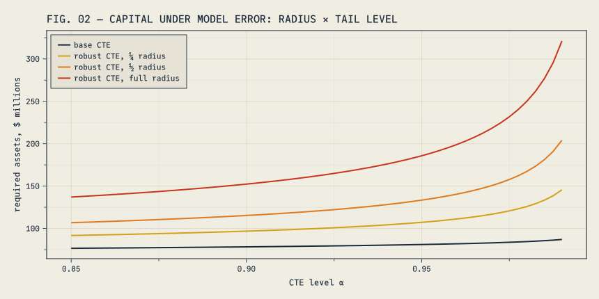
Now put those in dollars. The same $23.4M radius adds $74.1M of model-error charge at CTE(0.90), $104.7M at CTE(0.95), and $234.2M at CTE(0.99). Moving a capital standard from the 90th percentile to the 99th changes neither the model nor the radius, yet it roughly triples the price of every dollar of model error. And because the multiplier contains only \(\alpha\), none of this is a fact about our book. It is the same arithmetic for anyone whose capital metric lives deep in the tail of a model they know is imperfect.
FIG. 02 plotting code
let
    f = Figure(size = (860, 430))
    ax = Axis(f[1, 1], title = "FIG. 02 — CAPITAL UNDER MODEL ERROR: RADIUS × TAIL LEVEL",
        xlabel = "CTE level α", ylabel = "required assets, \$ millions")
    αs = range(0.85, 0.99; length = 57)
    base_curve = [CTE(α)(agg_current_basis) for α in αs]
    lines!(ax, αs, base_curve ./ 1e6; color = CF_INK, linewidth = 2.0, label = "base CTE")
    for (r, clr, lbl) in [(radius / 4, CF_AMBER, "robust CTE, ¼ radius"),
        (radius / 2, CF_ORANGE, "robust CTE, ½ radius"), (radius, CF_RED, "robust CTE, full radius")]
        lines!(ax, αs, [robustvalue(CTE(α), agg_current_basis; radius = r) for α in αs] ./ 1e6;
            color = clr, linewidth = 2.0, label = lbl)
    end
    axislegend(ax; position = :lt)
    f
end
FIG. 02 shows the same effect as curves. Follow the black base-CTE line first. It is nearly flat: with 1,775 expected claims a year, the aggregate distribution is close to symmetric, and raising \(\alpha\) from 0.85 to 0.99 adds only modestly to the base requirement. Now follow the three robust curves. They are not flat, and they spread apart as \(\alpha\) grows, because the model-error charge keeps rising with the multiplier even where the base curve has leveled off. Under model uncertainty, the choice of tail level does most of the work in setting the capital number.
Under the hood: where \((1-\alpha)^{-1/2}\) comes from. Sliding the worst \(1-\alpha\) slice of outcomes further out by the same amount \(\delta\) moves only a sliver of the distribution, so it is cheap: the \(W_2\) cost works out to \(\delta\sqrt{1-\alpha}\), because the rest of the distribution never moves. Spend the whole radius \(r\) and the slice slides out by \(\delta = r/\sqrt{1-\alpha}\) — which is exactly how much the tail average rises. The thinner the slice, the cheaper the attack and the longer the slide. A 99th-percentile promise concentrates everything in the thinnest slice, which is why it carries the largest multiplier.
Who sets the radius?
No theorem sets \(r\). What the formula gives back in exchange is linearity: half the radius, half the loading, so the ¼-, ½-, and full-radius columns of the table are the entire sensitivity analysis. Reasonable anchors, from harder to easier to argue with: the measured cost of one year of model movement, which is what we used — it prices staleness. The model-to-data misfit from part one, pushed through the same aggregate machine — the natural companion, because it prices exactly the shared structural error that a difference of two fits cancels; the two anchors answer complementary halves of “how wrong?”, the model lagging the world and the model missing the world. Or the rearrangement cost of a named scenario somebody in the room actually fears. Each produces a dollar figure a committee can dispute. The disputing is the point. The radius is where the judgment lives, and the table is what owning that judgment looks like.
What this doesn’t establish
In descending order of importance.
The worst case is conditional. Every robust number above is the worst among distributions within \(r\) of the fitted model. The truth has signed no agreement to stay in the ball.
The aggregate model is a model. Poisson counts, independence, a lognormal basis, frequency held fixed — the ball is drawn around all of those choices at once, and a radius calibrated from severity drift does not measure, say, frequency contagion or dependence across claimants.
The anchor is one observation, and a one-sided one. We watched the model move once and called that size a radius — an argument-starter, not a distribution of model error — and because the movement is a difference of two fits, error the fits share is invisible to it. A longer history, several scenarios priced the same way, or a misfit-based companion radius would anchor it better.
And everything is one-dimensional. The ball lives on the scalar annual total; the tail-slide inside robustvalue is one-dimensional to its bones. Joint moves — frequency with severity, several treaties at once — need multivariate transport, and the closed forms stop there.
The meeting, one floor up
The CFO’s question was: how wrong can the model be before the capital number is wrong too? Here is the answer with no theater in it. Base CTE(0.95), straight from the model: $81.1M. Measured movement of the model over one year: $23.4M. If next year’s model error is no bigger than that, the worst the true CTE(0.95) can be is $185.8M — base plus 4.47 for every dollar of radius, because that is what a 95th-percentile promise pays for model error. And one sentence rides along with the number: if the model is wrong by more than the radius, this figure promises nothing.
That sentence is the improvement. The old margin promised nothing either. It just never said so.
Further reading
- Daniel Kuhn, Peyman Mohajerin Esfahani, Viet Anh Nguyen & Soroosh Shafieezadeh-Abadeh (2019), Wasserstein Distributionally Robust Optimization — the theory behind the exact worst case, including the CTE stability bound used here.
- Arthur Charpentier (2026), Optimal Transport for Actuarial Science ⟨hal-05684645⟩ — a survey of transport ideas across actuarial problems; the package documentation follows it.
- ActuaryUtilities.jl risk measures documentation —
robustvalue, CTE, VaR, and exactly what is returned for measures without the closed form.
- How Far Did the Book Move? — part one: the drift measurement, its checks (a permutation screen and a generative Turing model), and the stress this post’s radius is anchored to.