Packages

JuliaActuary is an ecosystem of packages that makes Julia the easiest language to get started for actuarial workflows.

These packages are available for use in your project. Scroll down for more information and links to the associated repository for each one.

MortalityTables.jl Easily work with standard tables and parametric models with common survival calculations.	LifeContingencies.jl Insurance, annuity, premium, and reserve maths.
ActuaryUtilities.jl Robust and fast calculations for internal_rate_of_return, duration, convexity, present_value, breakeven, and more.	ExperienceAnalysis.jl Meeting your exposure calculation needs.
FinanceModels.jl Composable contracts, models, and functions that allow for modeling of both simple and complex financial instruments.	EconomicScenarioGenerators.jl Easy-to-use scenario generation that's FinanceModels.jl compatible.

Tip

For consistency, you can lock any package in its current state and not worry about breaking changes to any code that you write. Julia’s package manager lets you exactly recreate a set of code and its dependencies. More information.

Adding and Using Packages

There are two ways to add packages:

• In the code itself: using Pkg; Pkg.add("MortalityTables")
• In the REPL, hit ] to enter Pkg mode and type add MortalityTables More info can be found at the Pkg manager documentation.

To use packages in your code:

using PackageName

MortalityTables.jl

Hassle-free mortality and other rate tables.

Features

• Full set of SOA mort.soa.org tables included
• survival and decrement functions to calculate decrements over period of time
• Partial year mortality calculations (Uniform, Constant, Balducci)
• Friendly syntax and flexible usage
• Extensive set of parametric mortality models.

Quickstart

Load and see information about a particular table:

julia> vbt2001 = MortalityTables.table("2001 VBT Residual Standard Select and Ultimate - Male Nonsmoker, ANB")

MortalityTable (Insured Lives Mortality):
   Name:
       2001 VBT Residual Standard Select and Ultimate - Male Nonsmoker, ANB
   Fields:
       (:select, :ultimate, :metadata)
   Provider:
       Society of Actuaries
   mort.SOA.org ID:
       1118
   mort.SOA.org link:
       https://mort.soa.org/ViewTable.aspx?&TableIdentity=1118
   Description:
       2001 Valuation Basic Table (VBT) Residual Standard Select and Ultimate Table -  Male Nonsmoker.
       Basis: Age Nearest Birthday. 
       Minimum Select Age: 0. 
       Maximum Select Age: 99. 
       Minimum Ultimate Age: 25. 
       Maximum Ultimate Age: 120

The package revolves around easy-to-access vectors which are indexed by attained age:

julia> vbt2001.select[35]          # vector of rates for issue age 35
 0.00036
 0.00048
 ⋮
 0.94729
 1.0
 
julia> vbt2001.select[35][35]      # issue age 35, attained age 35
 0.00036
 
julia> vbt2001.select[35][50:end] # issue age 35, attained age 50 through end of table
0.00316
0.00345
 ⋮
0.94729
1.0

julia> vbt2001.ultimate[95]        # ultimate vectors only need to be called with the attained age
 0.24298

Calculate the force of mortality or survival over a range of time:

julia> survival(vbt2001.ultimate,30,40) # the survival between ages 30 and 40
0.9894404665434904

julia> decrement(vbt2001.ultimate,30,40) # the decrement between ages 30 and 40
0.010559533456509618

Non-whole periods of time are supported when you specify the assumption (Constant(), Uniform(), or Balducci()) for fractional periods:

julia> survival(vbt2001.ultimate,30,40.5,Uniform()) # the survival between ages 30 and 40.5
0.9887676470262408

Parametric Models

Over 20 different models included. Example with the Gompertz model

m = MortalityTables.Gompertz(a=0.01,b=0.2)

m[20]                 # the mortality rate at age 20
decrement(m,20,25)    # the five year cumulative mortality rate
survival(m,20,25) # the five year survival rate

MortalityTables package on Github 🡭

ActuaryUtilities.jl

A collection of common functions/manipulations used in Actuarial Calculations.

A collection of common functions/manipulations used in Actuarial Calculations.

Quickstart

cfs = [5, 5, 105]
times    = [1, 2, 3]

discount_rate = 0.03

present_value(discount_rate, cfs, times)           # 105.65
duration(Macaulay(), discount_rate, cfs, times)    #   2.86
duration(discount_rate, cfs, times)                #   2.78
convexity(discount_rate, cfs, times)               #  10.62

Features

Financial Maths

• duration:
  • Calculate the Macaulay, Modified, or DV01 durations for a set of cashflows
• convexity for price sensitivity
• Flexible interest rate options via the FinanceModels.jl package.
• internal_rate_of_return or irr to calculate the IRR given cashflows (including at timepoints like Excel’s XIRR)
• breakeven to calculate the breakeven time for a set of cashflows
• accum_offset to calculate accumulations like survivorship from a mortality vector

Options Pricing

• eurocall and europut for Black-Scholes option prices

Risk Measures

• Calculate risk measures for a given vector of risks:
  • CTE for the Conditional Tail Expectation, or
  • VaR for the percentile/Value at Risk.

Insurance mechanics

• duration:
  • Calculate the duration given an issue date and date (a.k.a. policy duration)

ActuaryUtilities package on GitHub 🡭

LifeContingencies.jl

Common life contingent calculations with a convenient interface.

Features

• Integration with other JuliaActuary packages such as MortalityTables.jl
• Fast calculations, with some parts utilizing parallel processing power automatically
• Use functions that look more like the math you are used to (e.g. A, ä) with Unicode support
• All of the power, speed, convenience, tooling, and ecosystem of Julia
• Flexible and modular modeling approach

Package Overview

• Leverages MortalityTables.jl for the mortality calculations
• Contains common insurance calculations such as:
  • Insurance(life,yield): Whole life
  • Insurance(life,yield,n): Term life for n years
  • ä(life,yield): present_value of life-contingent annuity
  • ä(life,yield,n): present_value of life-contingent annuity due for n years
• Contains various commutation functions such as D(x),M(x),C(x), etc.
• SingleLife and JointLife capable
• Interest rate mechanics via FinanceModels.jl
• More documentation available by clicking the DOCS badges at the top of this README

Examples

Basic Functions

Calculate various items for a 30-year-old male nonsmoker using 2015 VBT base table and a 5% interest rate

using LifeContingencies
using MortalityTables
using FinanceModels
import LifeContingencies: V, ä     # pull the shortform notation into scope

# load mortality rates from MortalityTables.jl
vbt2001 = MortalityTables.table("2001 VBT Residual Standard Select and Ultimate - Male Nonsmoker, ANB")

issue_age = 30
life = SingleLife(                 # The life underlying the risk
    mortality = vbt2001.select[issue_age],    # -- Mortality rates
)

yield = FinanceModels.Yield.Constant(0.05) 

lc = LifeContingency(life, yield)  # LifeContingency joins the risk with interest


ins = Insurance(lc)                # Whole Life insurance
ins = Insurance(life, yield)       # alternate way to construct

With the above life contingent data, we can calculate vectors of relevant information:

cashflows(ins)                     # A vector of the unit cashflows
timepoints(ins)                    # The timepoints associated with the cashflows
survival(ins)                      # The survival vector
benefit(ins)                       # The unit benefit vector
probability(ins)                   # The probability of benefit payment

Some of the above will return lazy results. For example, cashflows(ins) will return a Generator which can be efficiently used in most places you’d use a vector of cashflows (e.g. pv(...) or sum(...)) but has the advantage of being non-allocating (less memory used, faster computations). To get a computed vector instead of the generator, simply call collect(...) on the result: collect(cashflows(ins)).

Or calculate summary scalars:

present_value(ins)                 # The actuarial present value
premium_net(lc)                    # Net whole life premium 
V(lc,5)                            # Net premium reserve for whole life insurance at time 5

Other types of life contingent benefits:

Insurance(lc,10)                 # 10 year term insurance
AnnuityImmediate(lc)               # Whole life annuity due
AnnuityDue(lc)                     # Whole life annuity due
ä(lc)                              # Shortform notation
ä(lc, 5)                           # 5 year annuity due
ä(lc, 5, certain=5,frequency=4)    # 5 year annuity due, with 5 year certain payable 4x per year
...                                # and more!

Constructing Lives

SingleLife(vbt2001.select[50])                 # no keywords, just a mortality vector
SingleLife(vbt2001.select[50],issue_age = 60)  # select at 50, but now 60
SingleLife(vbt2001.select,issue_age = 50)      # use issue_age to pick the right select vector
SingleLife(mortality=vbt2001.select,issue_age = 50) # mort can also be a keyword

LifeContingencies package on GitHub 🡭

FinanceModels.jl

Flexible and composable yield curves and interest functions.

FinanceModels.jl provides a set of composable contracts, models, and functions that allow for modeling of both simple and complex financial instruments. The resulting models, such as discount rates or term structures, can then be used across the JuliaActuary ecosystem to perform actuarial and financial analysis.

Additionally, the models can be used to project contracts through time: most basically as a series of cashflows but more complex output can be defined for contracts.

Yields Curve Fitting in FinanceModels.jl

QuickStart

using FinanceModels

# a set of market-observed prices we wish to calibrate the model to
# annual effective unless otherwise specified
q_rate = ZCBYield([0.01,0.02,0.03]);
q_spread = ZCBYield([0.01,0.01,0.01]);

# bootstrap a linear spline yield model
model_rate = fit(Spline.Linear(),q_rate,Fit.Bootstrap());⠀           
model_spread = fit(Spline.Linear(),q_spread,Fit.Bootstrap());

# the zero rate is the combination of the two underlying rates
zero(m_spread + m_rate,1) # 0.02 annual effective rate 

# the discount is the same as if we added the underlying zero rates
discount(m_spread + m_rate,0,3) ≈ discount(0.01 + 0.03,3)   # true

# compute the present value of a contract (a cashflow of 10 at time 3)
present_value(m_rate,Cashflow(10,3)) # 9.15...

Overview of FinanceModels

A conceptual sketch of FinanceModels.jl

Often we start with observed or assumed values for existing contracts. We want to then use those assumed values to extend the valuation logic to new contracts. For example, we may have a set of bond yields which we then want to discount a series of insurance obligations.

In the language of FinanceModels, we would have a set of Quotes which are used to fit a Model. That model is then used to discount a new series of cashflows.

That’s just an example, and we can use the various components in different ways depending on the objective of the analysis.

Contracts and Quotes

Contracts are a way to represent financial obligations. These can be valued using a model, projected into a future steam of values, or combined with assumed prices as a Quote.

Included are a number of primitives and convenience methods for contracts:

Existing structs:

• Cashflow
• Bond.Fixed
• Bond.Floating
• Forward (an obligation with a forward start time)
• Composite (combine two other contracts, e.g. into a swap)
• EuroCall
• CommonEquity

Commonly, we deal with conventions that imply a contract and an observed price. For example, we may talk about a treasury yield of 0.03. This is a description that implies a Quoteed price for an underling fixed bond. In FinanceModels, we could use CMTYield(rate,tenor) which would create a Quote(price,Bond.Fixed(...)). In this way, we can conveniently create a number of Quotes which can be used to fit models. Such convenience methods include:

• ZCBYield
• ZCBPrice
• CMTYield
• ParYield
• ParSwapYield
• ForwardYield

FinanceModels offers a way to define new contracts as well.

Cashflows

A Cashflows obligation are themselves a contract, but other contracts can be considered as essentially anything that can be combined with assumptions (a model) to derive a collection of cashflows.

For example, a obligation that pays 1.75 at time 2 could be represented as: Cashflow(1.75,2).

Models

Models are objects that can be fit to observed prices and then subsequently used to make valuations of other cashflows/contracts.

Yield models include:

• Yield.Constant
• Bootstrapped Splines
• Yield.SmithWilson
• Yield.NelsonSiegel
• Yield.NelsonSiegelSvensson

Yield-related functions

The models can be used to compute various rates of interest:

• discount(curve,from,to) or discount(curve,to) gives the discount factor
• accumulation(curve,from,to) or accumulation(curve,to) gives the accumulation factor
• zero(curve,time) or zero(curve,time,Frequency) gives the zero-coupon spot rate for the given time.
• forward(curve,from,to) gives the zero rate between the two given times
• par(curve,time;frequency=2) gives the coupon-paying par equivalent rate for the given time.

Other models include:

• BlackScholesMerton derivative valuation

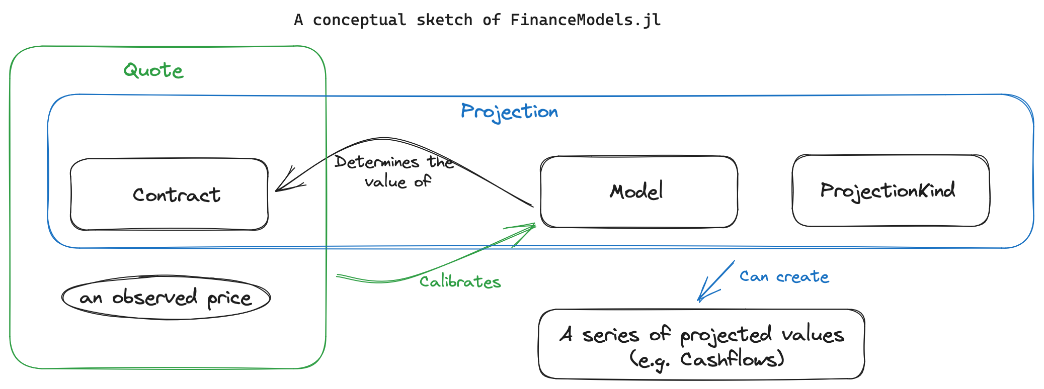
Projections

Most basically, we can project a contract into a series of Cashflows:

julia> b = Bond.Fixed(0.04,Periodic(2),3)
FinanceModels.Bond.Fixed{Periodic, Float64, Int64}(0.04, Periodic(2), 3)

julia> collect(b)
6-element Vector{Cashflow{Float64, Float64}}:
 Cashflow{Float64, Float64}(0.02, 0.5)
 Cashflow{Float64, Float64}(0.02, 1.0)
 Cashflow{Float64, Float64}(0.02, 1.5)
 Cashflow{Float64, Float64}(0.02, 2.0)
 Cashflow{Float64, Float64}(0.02, 2.5)
 Cashflow{Float64, Float64}(1.02, 3.0)

However, Projections allow one to combine three elements which can be extended to define any desired output (such as amortization schedules, financial statement projections, or account value rollforwards). The three elements are:

• the underlying contract of interest
• the model which includes assumptions of how the contract will behave
• a ProjectionKind which indicates the kind of output desired (cashflow stream, amortization schedule, etc…)

Fitting Models

       Model                                                               Method
          |                                                                   |
    |------------|                                                     |---------------|
fit(Spline.Cubic(), CMTYield.([0.04,0.05,0.055,0.06,0055],[1,2,3,4,5]), Fit.Bootstrap())
                    |-------------------------------------------------|
                                              |
                                              Quotes

• Model could be Spline.Linear(), Yield.NelsonSiegelSvensson(), Equity.BlackScholesMerton(...), etc.
• Quote could be CMTYields, ParYields, Option.Eurocall, etc.
• Method could be Fit.Loss(x->x^2), Fit.Loss(x->abs(x)), Fit.Bootstrap(), etc.

This unified way to fit models offers a much simpler way to extend functionality to new models or contract types.

Using Models

After being fit, models can be used to value contracts:

present_value(model,cashflows)

Additionally, ActuaryUtilities.jl offers a number of other methods that can be used, such as duration, convexity, price which can be used for analysis with the fitted models.

Rates

Rates are types that wrap scalar values to provide information about how to determine discount and accumulation factors.

There are two Frequency types:

• Periodic(m) for rates that compound m times per period (e.g. m times per year if working with annual rates).
• Continuous() for continuously compounding rates.

Examples

Continuous(0.05)       # 5% continuously compounded
Periodic(0.05,2)       # 5% compounded twice per period

These are both subtypes of the parent Rate type and are instantiated as:

Rate(0.05,Continuous())       # 5% continuously compounded
Rate(0.05,Periodic(2))        # 5% compounded twice per period

Rates can also be constructed by specifying the Frequency and then passing a scalar rate:

Periodic(1)(0.05)
Continuous()(0.05)

Conversion

Convert rates between different types with convert. E.g.:

r = Rate(FinanceModels.Periodic(12),0.01)             # rate that compounds 12 times per rate period (ie monthly)

convert(FinanceModels.Periodic(1),r)                  # convert monthly rate to annual effective
convert(FinanceModels.Continuous(),r)          # convert monthly rate to continuous

Arithmetic

Adding, substracting, multiplying, dividing, and comparing rates is supported.

FinanceModels package on GitHub 🡭

ExperienceAnalysis.jl

Meeting your exposure calculation needs.

Quickstart

df = DataFrame(
    policy_id = 1:3,
    issue_date = [Date(2020,5,10), Date(2020,4,5), Date(2019, 3, 10)],
    end_date = [Date(2022, 6, 10), Date(2022, 8, 10), Date(2022,12,31)],
    status = ["claim", "lapse", "inforce"]
)

df.policy_year = exposure.(
    ExperienceAnalysis.Anniversary(Year(1)),
    df.issue_date,
    df.end_date,
    df.status .== "claim"; # continued exposure
    study_start = Date(2020, 1, 1),
    study_end = Date(2022, 12, 31)
)

df = flatten(df, :policy_year)

df.exposure_fraction =
        map(e -> yearfrac(e.from, e.to + Day(1), DayCounts.Thirty360()), df.policy_year) 
# + Day(1) above because DayCounts has Date(2020, 1, 1) to Date(2021, 1, 1) as an exposure of 1.0
# here we end the interval at Date(2020, 12, 31), so we need to add a day to get the correct exposure fraction.

policy_id Int64	issue_date Date	end_date Date	status String	policy_year @NamedTuple{from::Date, to::Date, policy\_timestep::Int64}	exposure_fraction Float64
1	2020-05-10	2022-06-10	claim	(from = Date(“2020-05-10”), to = Date(“2021-05-09”), policy_timestep = 1)	1.0
1	2020-05-10	2022-06-10	claim	(from = Date(“2021-05-10”), to = Date(“2022-05-09”), policy_timestep = 2)	1.0
1	2020-05-10	2022-06-10	claim	(from = Date(“2022-05-10”), to = Date(“2023-05-09”), policy_timestep = 3)	1.0
2	2020-04-05	2022-08-10	lapse	(from = Date(“2020-04-05”), to = Date(“2021-04-04”), policy_timestep = 1)	1.0
2	2020-04-05	2022-08-10	lapse	(from = Date(“2021-04-05”), to = Date(“2022-04-04”), policy_timestep = 2)	1.0
2	2020-04-05	2022-08-10	lapse	(from = Date(“2022-04-05”), to = Date(“2022-08-10”), policy_timestep = 3)	0.35
3	2019-03-10	2022-12-31	inforce	(from = Date(“2020-01-01”), to = Date(“2020-03-09”), policy_timestep = 1)	0.191667
3	2019-03-10	2022-12-31	inforce	(from = Date(“2020-03-10”), to = Date(“2021-03-09”), policy_timestep = 2)	1.0
3	2019-03-10	2022-12-31	inforce	(from = Date(“2021-03-10”), to = Date(“2022-03-09”), policy_timestep = 3)	1.0
3	2019-03-10	2022-12-31	inforce	(from = Date(“2022-03-10”), to = Date(“2022-12-31”), policy_timestep = 4)	0.808333

Available Exposure Basis

• ExperienceAnalysis.Anniversary(period) will give exposures periods based on the first date
• ExperienceAnalysis.Calendar(period) will follow calendar periods (e.g. month or year)
• ExperienceAnalysis.AnniversaryCalendar(period,period) will split into the smaller of the calendar or policy period.

Where period is a Period Type from the Dates standard library.

Calculate exposures with exposures(basis,from,to,continue_exposure).

• continue_exposures indicates whether the exposure should be extended through the full exposure period rather than terminate at the to date.

ExperienceAnalysis package on GitHub 🡭

EconomicScenarioGenerators.jl

Easy-to-use scenario generation that’s FinanceModels.jl compatible.

Models

Interest Rate Models

• Vasicek
• CoxIngersolRoss
• HullWhite

EquityModels

• BlackScholesMerton

Interest Rate Model Examples

Vasicek

m = Vasicek(0.136,0.0168,0.0119,Continuous(0.01)) # a, b, σ, initial Rate
s = ScenarioGenerator(
        1,  # timestep
        30, # projection horizon
        m,  # model
    )

This can be iterated over, or you can collect all of the rates like:

rates = collect(s)

or

for r in s
    # do something with r
end

And the package integrates with FinanceModels.jl:

YieldCurve(s)

will produce a yield curve object:

              ⠀⠀⠀⠀⠀⠀⠀⠀⠀⠀⠀⠀⠀⠀Yield Curve (FinanceModels.BootstrapCurve)⠀⠀⠀⠀⠀⠀⠀⠀⠀⠀⠀⠀⠀           
              ┌────────────────────────────────────────────────────────────┐           
         0.03 │⠀⠀⠀⠀⠀⠀⠀⠀⠀⠀⠀⠀⠀⠀⠀⠀⠀⠀⠀⠀⠀⠀⠀⠀⠀⠀⠀⠀⠀⠀⠀⠀⠀⠀⠀⠀⠀⠀⠀⠀⠀⠀⠀⠀⠀⣀⠤⠤⠔⠒⠉⠉⠒⠒⠒⠒⠒⠤⣄⣀│ Zero rates
              │⠀⠀⠀⠀⠀⠀⠀⠀⠀⠀⠀⠀⠀⠀⠀⠀⠀⠀⠀⠀⠀⠀⠀⠀⠀⠀⠀⠀⠀⠀⠀⠀⠀⠀⠀⠀⠀⠀⠀⠀⣀⠤⠒⠒⠉⠀⠀⠀⠀⠀⠀⠀⠀⠀⠀⠀⠀⠀⠀⠀│           
              │⠀⠀⠀⠀⠀⠀⠀⠀⠀⠀⠀⠀⠀⠀⠀⠀⠀⠀⠀⠀⠀⠀⠀⠀⠀⠀⠀⠀⠀⠀⠀⠀⠀⠀⠀⠀⠀⣀⠔⠊⠁⠀⠀⠀⠀⠀⠀⠀⠀⠀⠀⠀⠀⠀⠀⠀⠀⠀⠀⠀│           
              │⠀⠀⠀⠀⠀⠀⠀⠀⠀⠀⠀⠀⠀⠀⠀⠀⠀⠀⠀⠀⠀⠀⠀⠀⠀⠀⠀⠀⠀⠀⠀⠀⠀⠀⣀⠔⠋⠁⠀⠀⠀⠀⠀⠀⠀⠀⠀⠀⠀⠀⠀⠀⠀⠀⠀⠀⠀⠀⠀⠀│           
              │⠀⠀⠀⠀⠀⠀⠀⠀⠀⠀⠀⠀⠀⠀⠀⠀⠀⠀⠀⠀⠀⠀⠀⠀⢀⣀⣀⠀⠀⣀⡤⠖⠊⠉⠀⠀⠀⠀⠀⠀⠀⠀⠀⠀⠀⠀⠀⠀⠀⠀⠀⠀⠀⠀⠀⠀⠀⠀⠀⠀│           
              │⠀⠀⠀⠀⠀⠀⠀⠀⠀⠀⠀⠀⠀⠀⠀⠀⠀⠀⠀⠀⣀⠤⠖⠋⠁⠀⠀⠉⠉⠁⠀⠀⠀⠀⠀⠀⠀⠀⠀⠀⠀⠀⠀⠀⠀⠀⠀⠀⠀⠀⠀⠀⠀⠀⠀⠀⠀⠀⠀⠀│           
              │⠀⠀⠀⠀⠀⠀⠀⠀⠀⠀⠀⠀⠀⠀⠀⠀⠀⣀⠔⠋⠀⠀⠀⠀⠀⠀⠀⠀⠀⠀⠀⠀⠀⠀⠀⠀⠀⠀⠀⠀⠀⠀⠀⠀⠀⠀⠀⠀⠀⠀⠀⠀⠀⠀⠀⠀⠀⠀⠀⠀│           
   Continuous │⠀⠀⠀⠀⠀⠀⠀⠀⠀⣀⡤⠒⠓⠦⠤⠖⠉⠀⠀⠀⠀⠀⠀⠀⠀⠀⠀⠀⠀⠀⠀⠀⠀⠀⠀⠀⠀⠀⠀⠀⠀⠀⠀⠀⠀⠀⠀⠀⠀⠀⠀⠀⠀⠀⠀⠀⠀⠀⠀⠀│           
              │⠀⠀⠀⠀⠀⠀⠀⢰⠋⠁⠀⠀⠀⠀⠀⠀⠀⠀⠀⠀⠀⠀⠀⠀⠀⠀⠀⠀⠀⠀⠀⠀⠀⠀⠀⠀⠀⠀⠀⠀⠀⠀⠀⠀⠀⠀⠀⠀⠀⠀⠀⠀⠀⠀⠀⠀⠀⠀⠀⠀│           
              │⠀⠀⣀⠖⠢⡀⡰⠃⠀⠀⠀⠀⠀⠀⠀⠀⠀⠀⠀⠀⠀⠀⠀⠀⠀⠀⠀⠀⠀⠀⠀⠀⠀⠀⠀⠀⠀⠀⠀⠀⠀⠀⠀⠀⠀⠀⠀⠀⠀⠀⠀⠀⠀⠀⠀⠀⠀⠀⠀⠀│           
              │⠉⠉⠁⠀⠀⠉⠁⠀⠀⠀⠀⠀⠀⠀⠀⠀⠀⠀⠀⠀⠀⠀⠀⠀⠀⠀⠀⠀⠀⠀⠀⠀⠀⠀⠀⠀⠀⠀⠀⠀⠀⠀⠀⠀⠀⠀⠀⠀⠀⠀⠀⠀⠀⠀⠀⠀⠀⠀⠀⠀│           
              │⠀⠀⠀⠀⠀⠀⠀⠀⠀⠀⠀⠀⠀⠀⠀⠀⠀⠀⠀⠀⠀⠀⠀⠀⠀⠀⠀⠀⠀⠀⠀⠀⠀⠀⠀⠀⠀⠀⠀⠀⠀⠀⠀⠀⠀⠀⠀⠀⠀⠀⠀⠀⠀⠀⠀⠀⠀⠀⠀⠀│           
              │⠀⠀⠀⠀⠀⠀⠀⠀⠀⠀⠀⠀⠀⠀⠀⠀⠀⠀⠀⠀⠀⠀⠀⠀⠀⠀⠀⠀⠀⠀⠀⠀⠀⠀⠀⠀⠀⠀⠀⠀⠀⠀⠀⠀⠀⠀⠀⠀⠀⠀⠀⠀⠀⠀⠀⠀⠀⠀⠀⠀│           
              │⠀⠀⠀⠀⠀⠀⠀⠀⠀⠀⠀⠀⠀⠀⠀⠀⠀⠀⠀⠀⠀⠀⠀⠀⠀⠀⠀⠀⠀⠀⠀⠀⠀⠀⠀⠀⠀⠀⠀⠀⠀⠀⠀⠀⠀⠀⠀⠀⠀⠀⠀⠀⠀⠀⠀⠀⠀⠀⠀⠀│           
            0 │⠀⠀⠀⠀⠀⠀⠀⠀⠀⠀⠀⠀⠀⠀⠀⠀⠀⠀⠀⠀⠀⠀⠀⠀⠀⠀⠀⠀⠀⠀⠀⠀⠀⠀⠀⠀⠀⠀⠀⠀⠀⠀⠀⠀⠀⠀⠀⠀⠀⠀⠀⠀⠀⠀⠀⠀⠀⠀⠀⠀│           
              └────────────────────────────────────────────────────────────┘           
              ⠀0⠀⠀⠀⠀⠀⠀⠀⠀⠀⠀⠀⠀⠀⠀⠀⠀⠀⠀⠀⠀⠀⠀⠀⠀⠀⠀time⠀⠀⠀⠀⠀⠀⠀⠀⠀⠀⠀⠀⠀⠀⠀⠀⠀⠀⠀⠀⠀⠀⠀⠀⠀⠀⠀30⠀           

EconomicScenarioGenerators package on GitHub 🡭