Fitting Rate Data to Yield Curves

Given rates and maturities, we can fit the yield curves with different techniques.

Below, we specify that the rates should be interpreted as Continuously compounded zero rates:

using FinanceModels
using CairoMakie

# Apply the site's custom Makie plot theme (cassette futurism).
include(joinpath(@__DIR__, "..", "..", "assets", "themes", "cassette_futurism.jl"))
set_theme!(cassette_futurism_theme())

rates = Continuous.([0.01, 0.01, 0.03, 0.05, 0.07, 0.16, 0.35, 0.92, 1.40, 1.74, 2.31, 2.41] ./ 100)
mats = [1 / 12, 2 / 12, 3 / 12, 6 / 12, 1, 2, 3, 5, 7, 10, 20, 30]

12-element Vector{Float64}:
  0.08333333333333333
  0.16666666666666666
  0.25
  0.5
  1.0
  2.0
  3.0
  5.0
  7.0
 10.0
 20.0
 30.0

The above rates and associated maturities represent yields of zero coupon bonds (from which the corresponding prices follow), which we use as the financial instrument that we will fit the curve to:

quotes = ZCBYield.(rates, mats)

12-element Vector{Quote{Float64, Cashflow{Float64, Float64}}}:
 Quote{Float64, Cashflow{Float64, Float64}}(0.9999916667013888, Cashflow{Float64, Float64}(1.0, 0.08333333333333333))
 Quote{Float64, Cashflow{Float64, Float64}}(0.9999833334722215, Cashflow{Float64, Float64}(1.0, 0.16666666666666666))
 Quote{Float64, Cashflow{Float64, Float64}}(0.9999250028124297, Cashflow{Float64, Float64}(1.0, 0.25))
 Quote{Float64, Cashflow{Float64, Float64}}(0.999750031247396, Cashflow{Float64, Float64}(1.0, 0.5))
 Quote{Float64, Cashflow{Float64, Float64}}(0.9993002449428433, Cashflow{Float64, Float64}(1.0, 1.0))
 Quote{Float64, Cashflow{Float64, Float64}}(0.9968051145430329, Cashflow{Float64, Float64}(1.0, 2.0))
 Quote{Float64, Cashflow{Float64, Float64}}(0.9895549325678993, Cashflow{Float64, Float64}(1.0, 3.0))
 Quote{Float64, Cashflow{Float64, Float64}}(0.9550419621907147, Cashflow{Float64, Float64}(1.0, 5.0))
 Quote{Float64, Cashflow{Float64, Float64}}(0.9066489037539209, Cashflow{Float64, Float64}(1.0, 7.0))
 Quote{Float64, Cashflow{Float64, Float64}}(0.8402968976584314, Cashflow{Float64, Float64}(1.0, 10.0))
 Quote{Float64, Cashflow{Float64, Float64}}(0.6300223399419124, Cashflow{Float64, Float64}(1.0, 20.0))
 Quote{Float64, Cashflow{Float64, Float64}}(0.4852941873885002, Cashflow{Float64, Float64}(1.0, 30.0))

With FinanceModels 7, Fit.Bootstrap() supports linear interpolation. Quadratic and cubic splines use a loss fit over all quotes. Here are six alternatives:

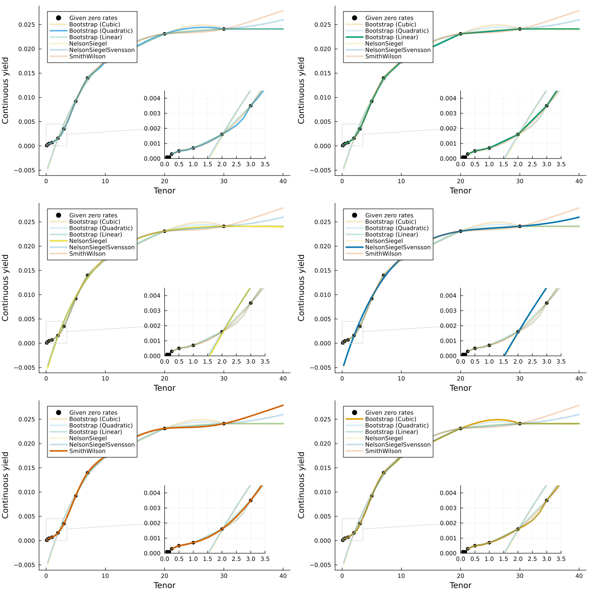
ns = fit(Yield.NelsonSiegel(), quotes);
nss = fit(Yield.NelsonSiegelSvensson(), quotes);
sw = fit(Yield.SmithWilson(ufr=0.05, α=0.1), quotes);
bl = fit(Spline.Linear(), quotes, Fit.Bootstrap());
bq = fit(Spline.Quadratic(), quotes, Fit.Loss(x -> x^2));
bc = fit(Spline.Cubic(), quotes, Fit.Loss(x -> x^2));

These curves can discount cashflows with present_value, or supply duration and convexity calculations in ActuaryUtilities. The fitted spline curves use flat-forward extrapolation after the final 30-year knot. Their zero rates approach that forward rate; they do not continue the final interpolation polynomial.

For direct interpolation of observed zero rates, use ZeroRateCurve(rates, mats, Spline.Cubic()). A loss fit is useful when fitting the prices of coupon-bearing instruments as well.

Visualizing the results

const CURVES = [
    (bc,  "Loss fit (Cubic)"),
    (bq,  "Loss fit (Quadratic)"),
    (bl,  "Bootstrap (Linear)"),
    (ns,  "NelsonSiegel"),
    (nss, "NelsonSiegelSvensson"),
    (sw,  "SmithWilson"),
]

function curveplot!(ax, curve, color; label="", alpha=1.0)
    maturities = 0.25:0.25:40
    f(x) = rate(zero(curve, x))
    lines!(ax, maturities, f.(maturities);
        label, linewidth=3, color=(color, alpha))
end

function build_axis!(ax, alpha=ones(length(CURVES)))
    scatter!(ax, mats, rate.(Continuous().(rates));
        label="Given zero rates", color=CF_INK, markersize=9)
    for (i, (c, name)) in enumerate(CURVES)
        curveplot!(ax, c, CASSETTE_PALETTE[i]; label=name, alpha=alpha[i])
    end
    return ax
end

let
    fig = Figure(size=(760, 460))
    ax = Axis(fig[1,1]; xlabel="Tenor", ylabel="Continuous yield")
    build_axis!(ax)
    axislegend(ax, position=:lt)
    fig
end

Fitted yield curves across tenors, compared with the observed continuously compounded zero rates.

And an animated version that fades each fit in turn:

let
    fig = Figure(size=(760, 460))
    ax = Axis(fig[1,1]; xlabel="Tenor", ylabel="Continuous yield")
    a = [1.0, 0.25, 0.25, 0.25, 0.25, 0.25]
    record(fig, "anim_fps2.gif", 1:6; framerate=2) do _
        a .= circshift(a, 1)
        empty!(ax)
        build_axis!(ax, a)
        axislegend(ax, position=:lt)
    end
end