Current package benchmarks
The fall 2026 release benchmarks compare FinanceCore 3, FinanceModels 7, ActuaryUtilities 6 and MortalityTables 3 with the preceding releases. They include scripts, environments and raw results, with Julia timings taken from the minimum of warmed BenchmarkTools trials across repeated runs. The QuantLib comparison covers matched cashflow and sensitivity calculations.
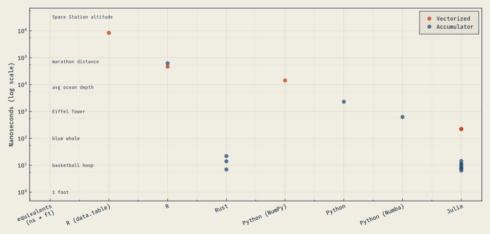
The cross-language measurements below are historical results from the linked benchmark studies. They have not been rerun for the current package releases; their speed ratios describe those original environments.
The Life Modeling Problem
Inspired by the discussion in the ActuarialOpenSource GitHub community discussion, folks started submitted solutions to what someone referred to as the “Life Modeling Problem”. This user submitted a short snippet for consideration of a representative problem.
Benchmarks
After the original user submitted a proposal, others chimed in and submitted versions in their favorite languages. I have collected those versions, and run them on a consistent set of hardware.
Some submissions were excluded because from the benchmarks they involved an entirely different approach, such as memoizing the function calls.
To aid in visualizing results with such vast different orders of magnitude, this graph includes a physical length comparison to serve as a reference. The computation time is represented by the distance that light travels in the time for the computation to complete (comparing a nanosecond to one foot length goes at least back to Admiral Grace Hopper).
Discussion
For more a more in-depth discussion of these results, see this post.
All of the benchmarked code can be found in the JuliaActuary Learn repository. Please file an issue or submit a PR request there for issues/suggestions.
IRRs
Task: determine the IRR for a series of cashflows 701 elements long (roughly 58 years of monthly cashflows).
Benchmarks
Times are in nanoseconds:
┌──────────┬──────────────────┬───────────────────┬─────────┬─────────────┬───────────────┐
│ Language │          Package │          Function │  Median │        Mean │ Relative Mean │
├──────────┼──────────────────┼───────────────────┼─────────┼─────────────┼───────────────┤
│   Python │  numpy_financial │               irr │ missing │   519306422 │       123146x │
│   Python │           better │ irr_binary_search │ missing │     3045229 │          722x │
│   Python │           better │        irr_newton │ missing │      382166 │           91x │
│    Julia │ ActuaryUtilities │               irr │    4185 │        4217 │            1x │
└──────────┴──────────────────┴───────────────────┴─────────┴─────────────┴───────────────┘
Discussion
The ActuaryUtilities implementation is over 100,000 times faster than numpy_financial, and 91 to 722 times faster than the better Python package. The ActuaryUtilities.jl implementation is also more flexible, as it can be given an argument with timepoints, similar to Excel’s XIRR.
Excel was used to attempt a benchmark, but the IRR formula returned a #DIV/0! error.
All of the benchmarked code can be found in the JuliaActuary Learn repository. Please file an issue or submit a PR request there for issues/suggestions.
Black-Scholes-Merton European Option Pricing
Task: calculate the price of a vanilla european call option using the Black-Scholes-Merton formula.
\[\begin{align}
C(S_t, t) &= N(d_1)S_t - N(d_2)Ke^{-r(T - t)} \\
d_1 &= \frac{1}{\sigma\sqrt{T - t}}\left[\ln\left(\frac{S_t}{K}\right) + \left(r + \frac{\sigma^2}{2}\right)(T - t)\right] \\
d_2 &= d_1 - \sigma\sqrt{T - t}
\end{align}\]
Benchmarks
Times are in nanoseconds:
┌──────────┬─────────┬─────────────┬───────────────┐
│ Language │  Median │        Mean │ Relative Mean │
├──────────┼─────────┼─────────────┼───────────────┤
│   Python │ missing │    817000.0 │       19639.4 │
│        R │  3649.0 │      3855.2 │          92.7 │
│    Julia │    41.0 │        41.6 │           1.0 │
└──────────┴─────────┴─────────────┴───────────────┘
Discussion
Julia is nearly 20,000 times faster than Python, and two orders of magnitude faster than R.
Nested Stochastic Projections
Task: value a 190,000-policy variable annuity block (GMWB/GMDB/GMMB riders) by full brute force — 1,000 outer real-world scenarios × 500 inner risk-neutral scenarios at each of 120 quarterly switch points, about \(10^{13}\) path valuations — reproducing the reference model of the SOA’s 2021 Efficient Computational Structure of Nested Stochastic Modeling paper exactly.
Discussion
Translating the Python line-for-line into Julia is worth ~90X on the naive loops and ~2.7X on the completed NumPy/RISP version. Restructuring into a fused seriatim kernel — about 40 lines that read like the model specification and reproduce every other implementation’s numbers to ~1e-11 or better — is worth ~110X over the completed NumPy version on the same laptop, largely by skipping work (each policy stops at its own maturity) and threading freely. The same kernel, moved to a rented H100 via KernelAbstractions.jl, ran the paper’s full “560-day” configuration in 24.8 measured minutes (~$1 of compute) — roughly 1,000X more throughput per unit of work than CuPy on the same GPU, whose array formulation is launch-overhead-bound.
For the full ladder, cross-implementation validation, pathwise AD sensitivities, and the GPU details — plus the archived code and results — see the post.
Other benchmarks
These benchmarks have been performed by others, but provide relevant information for actuarial-related work:
Colophon
Code
All of the benchmarked code can be found in the JuliaActuary Learn repository. Please file an issue or submit a PR request there for issues/suggestions.