Fitting Yield Curves to rates

Given rates and maturities, we can fit the yield curves with different techniques in Yields.jl.

Below, we specify that the rates should be interpreted as Continuously compounded zero rates:

using FinanceModels, FinanceCore

rates = Continuous.([0.01, 0.01, 0.03, 0.05, 0.07, 0.16, 0.35, 0.92, 1.40, 1.74, 2.31, 2.41] ./ 100)
mats = [1/12, 2/12, 3/12, 6/12, 1, 2, 3, 5, 7, 10, 20, 30]

quotes = ZCBYield.(rates,mats)

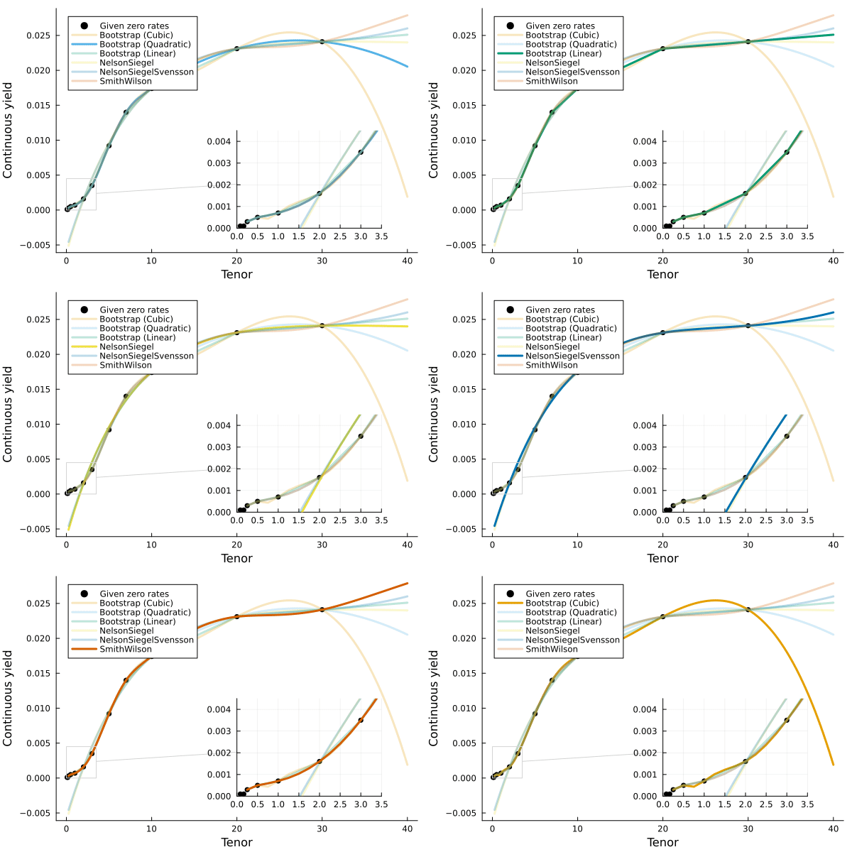
Then fit the rates under six methods:

• Nelson-Siegel

• Nelson-Siegel-Svensson

• Smith-Wilson

• Bootstrapping with linear splines

• Bootstrapping with quadratic splines

• Bootstrapping with cubic splines

ns =  fit(Yield.NelsonSiegel(),              quotes)
nss = fit(Yield.NelsonSiegelSvensson(),      quotes)
nss = fit(Yield.SmithWilson(ufr=0.05,α=0.1), quotes)
bl =  fit(Spline.Linear(),                   quotes, Fit.Bootstrap())
bq =  fit(Spline.Quadratic(),                quotes, Fit.Bootstrap())
bc =  fit(Spline.Cubic(),                    quotes, Fit.Bootstrap())

That's it! We've used the FinanceModels.jl fit method to construct yield curves using four different techniques. These can now be used in a variety of ways, such as calculating the present_value, duration, or convexity of different cashflows if you imported ActuaryUtilities.jl

A visualization of the different curves:

Associated Pluto Notebook

This example, complete with the code to plot/animate the curves is in the notebook below. To use Pluto to run the notebook:

1. Open a Julia REPL and copy and paste the following:

# install these dependencies
import Pkg; Pkg.add("Pluto") 

# use and start Pluto
using Pluto; Pluto.run()

2. In the Pluto window that opens, enter this URL into the Open from file: box:

https://raw.githubusercontent.com/JuliaActuary/Learn/master/Yield_Curve_fitting.jl